Hamiltonian Monte Carlo for Babies

Foreword

This semester, the instructor of the intro-level Bayesian Statistics course in my department decided to convert all students into using stan for statistical computing. From a Bayesian statistician’s perspective, stan is a really great tool for MCMC (Markov chain Monte Carlo) sampling, but it uses something called “Hamiltonian Monte Carlo” (HMC) which is not easy to understand or explain.

Well, it definitely took me a while to kind of (but not exactly) get what HMC is and why it works so well. AND I had to teach a roomful of PhD students about it in a lab session! So, after quite some struggling, I did manage to give a mini lecture on this topic, and this blog post is a compilation of my (very short) lecture notes.

Almost all the materials here are from this very well-written article by Michael Betancourt and this great YouTube playlist by Gabriele Carcassi. My “baby” version is obviously much less rigorous (and shorter!), but hopefully I can convey the basic message.

Conventional MCMC methods sometimes don’t work

Many of us (including me) have used and love to use methods like Gibbs sampling or Metropolis-Hastings sampling. These methods are often (relatively) easy to understand, formulate, and programme, but unfortunately they perform unsatisfactorily when the target density (e.g. posterior density) looks “weird” or “ugly”.

So, they work fine when the target density looks nice and smooth like this one.

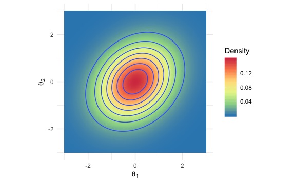
But they really struggle when the density looks like this ugly-shaped thing; there are two narrow, sharp ridges on the density surface, which a usual MCMC sampler either cannot reach or cannot escape once inside.

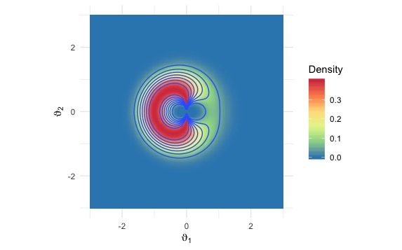
(Both pictures are drawn by Jordan Bryan, a brilliant colleague of mine.)

For example, Gibbs samplers often suffer from these two major issues:

• High autocorrelation; this leads to “sticky” chains and very low effective sample sizes.
• Getting “stuck”; when the target density has high curvature regions, the sampler tends to get trapped in those regions.

And that’s why certain smart people started searching for alternative sampling methods that can handle tricky densities. (Then they found out the magical Hamiltonian Monte Carlo and built stan.)

HMC tackles “weird” densities via “nice” Markov Chain transitions

The key idea of MCMC sampling is to “walk around” the parameter space according to the target density; if you do it right and long enough, eventually you get a bunch of samples with an empirical distribution just like your target density.

Therefore in MCMC, two things have to work out:

• We need to sample from the “right” region
• We need to “fully explore” the sample space

Correspondingly, a good MCMC sampling method should be able to:

• Quickly find the “right” region; this is not just the high density region, but rather a broader area with not-too-low densities (the so-called “typical set”)
• Efficiently move around within the right region; this means it must have a “nice” way to transition from one spot to another

As it turns out, HMC ticks both boxes (hooray!).

It sounds like a myth, but HMC does stand on solid theoretical grounds in differential geometry. Unfortunately “differential geometry” is something way too dense for an average statistician, but, fortunately, its intuition can be gained from Hamiltonian mechanics.

HMC and Hamiltonian mechanics: why it works

(I’m assuming that you still remember a bit of high school physics…)

Hamiltonian mechanics for babies (with a high school diploma)

Very loosely speaking, Hamiltonian mechanics describes the mechanics in an ideal world where the total volume of mechanic energy is preserved.

Imagine we are riding a little shuttle in this cute, ideal world. Let \(x\) represent our location and \(p\) represent our momentum (this is just mass multiplied by velocity). So, in some sense, the location \(x\) relates to our potential energy, \(V(x)\), and the momentum \(p\) relates to our kinetic energy, \(K(p,x)\) (let it somehow depend on the location too).

Let us call the total mechanic energy \(H(p,x)\) (the “Hamiltonian”), that is, \[ H(p,x) = K(p,x) + V(x).\]

Since the mechanic energy is preserved, \(H(p,x)\) remains the same. And therefore if we toggle our momentum \(p\) somehow, \(K(p,x)\) gets changed, which leads to the same amount of change (albeit in the opposite direction) in \(V(x)\), and that drives us to a different location \(x\).

In fact, in Hamiltonian mechanics, there is a set of differential equations that deterministically tell us how \(p\) and \(x\) evolve through time, and thus tell us how our shuttle travels around the space. (See the next section for details.)

Back to the sampling world

Now, let’s map this back to statistical terms.

Suppose \(\pi(x)\) is the target density, so what we want is to sample a bunch of \(x\) values according to \(\pi(x)\). In HMC, each entry of \(x\) (yes, \(x\) can be multi-dimensional!) is paired with a momentum, which gives us the auxiliary momenta \(p\). Take the negative logarithm of the target density and take the resulting function as the “potential energy” function. Then, a fitting “kinetic energy” function is found for the momenta \(p\) and original parameter \(x\), and that is in turn the negative logarithm of some conditional density function for \(p\), \(\pi_0(p \mid x)\).

To clarify, we are basically mapping probabilistic densities into “energies”:

• \(-\log \pi(x) \rightarrow V(x)\); target density \(\rightarrow\) potential energy
• \(-\log \pi_0(p \mid x) \rightarrow K(p,x)\); auxiliary density \(\rightarrow\) kinetic energy

So for the joint density of \(x\) and \(p\), \(\pi_1 (p, x) = \pi_0(p\lvert x) \pi(x) \), its negative logarithm can thus be mapped to the total mechanic energy, the Hamiltonian: \[ -\log \pi_1 (p, x) = -\log (\pi_0(p \mid x) \pi(x)) = -\log \pi_0(p \mid x) -\log \pi(x) \rightarrow K(p,x) + V(x) = H(p,x).\]

Following the “toggle momentum” argument aforementioned, toggling the auxiliary parameters \(p\) helps us move around the space of \(x\), and by the properties of Hamiltonian mechanics, the way we get to move around (the “transition”) can:

• drive us (rapidly) to the “right” region of the parameter space, and
• traverse within the “right” region and fully explore

And lo and behold, these two things match up with what we expect from a good MCMC sampler!

HMC’s “nice” transitions

Let us look a bit more closely at how “nicely” HMC moves around the parameter space.

HMC trajectories are driven by target gradient, but not entirely

In Hamiltonian mechanics, the trajectories (over time) of the momentum \(p\) and location \(x\) are governed by the Hamiltonian equations:

When mapping back to probabilistic densities:

We can see (in the second equation) that the movement of \(p\) is partially driven by the gradient of the log-density function \(\log\pi(x)\). That means the trajectories in HMC lead us towards regions with relatively high density, but also avoid crashing straight into a high density region and getting stuck there.

Independence across dimensions

Another quite interesting property of Hamiltonian mechanics is that the total energy is preserved along every dimension. This implies that the movements of \(p\) and \(x\) are independent across dimensions. More specifically, the exploration of \((p_i, x_i)\) does not get in the way of the exploration of \((p_j, x_j)\) (\(i \neq j\)).

Recall that in Gibbs sampling, we sample from the full conditional distributions \[p(x_i \mid \text{all other } x_j’s),\] and that means our movement along the \(i\)’s dimension is restricted by our locations on all the other dimensions, which can lead to pathological behaviors when the target density is “ugly” (like the one in the second graph up front).

HMC, however, doesn’t suffer from this problem.

Major takeaway

Hamiltonian Monte Carlo is a conceptually complicated statistical computing method, but in practice it works really well.

So, when things go sideways with your old-school Gibbs sampler, maybe try out HMC using softwares like stan.